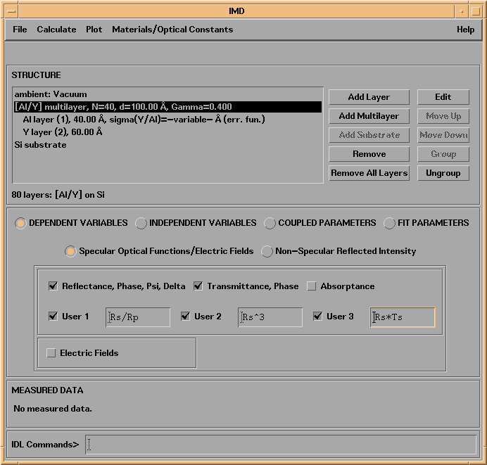
Specifying dependent variables - the optical functions you wish to compute - is simple: just click on the desired variables in the DEPENDENT VARIABLES area of the main IMD widget:
SPECULAR OPTICAL FUNCTIONS / ELECTRIC FIELDS
Figure 2.1 shows the main IMD widget as it appears when the DEPENDENT VARIABLES button is selected, and the Specular Optical Functions / Electric Fields button is selected. Select whichever functions you wish to compute.
Note that for each specular optical function you select, the program will calculate the values of that property for pure s and pure p polarization, as well as the average value of the property for the specified polarization parameters f and q (described below). For instance, if you select reflectance as a dependent variable, when you actually perform the calculation the program will compute the reflectances for pure s and p polarization, R(s), and R(p), in addition to the average reflectance R(f,q). In the case of reflectance and transmittance, the program will also compute the phases of the reflected and/or transmitted waves for pure s and pure p polarizations; the ellipsometric psi and delta functions will be computed as well if Reflectance is selected as a dependent variable. Once the calculation is performed, any or all of these variables can be displayed.
USER-DEFINED SPECULAR OPTICAL FUNCTIONS
Once you have selected any specular optical functions (reflectance, transmittance, and/or absorptance) as dependent variables, you can also choose to calculate up to three so-called 'user-defined' optical functions. These functions are completely arbitrary combinations of whatever optical functions you're interested in. For example, to compute the ratio of reflectance for pure s to pure p polarization, you can define a user-function equal to Rs/Rp, as shown in Figure 2.3.1 (i.e., the User 1 function):
Figure 2.3.1 The main IMD widget, showing some user-defined function examples.

User-functions can make use of any of the specular optical functions you wish to calculate, and can also use any other valid IDL functions. The only constraints are that (a) you must use valid IDL syntax, (b) you must use the correct variable names of any IMD optical functions you reference, and (c) the user-functions you calculate must have the same dimensionality as all the other optical functions for a given calculation (an example of an invalid user function is total(Rs), which is a scalar.)
Consult Appendix B.4 for a complete listing of all the IMD specular optical function variable names available for use in user-defined functions.
NON-SPECULAR OPTICAL FUNCTIONS
The non-specular (i.e., diffuse) reflected intensity from a multilayer film can be computed using either a dynamical Born approximation (BA) vector theory, described in reference [4], or the so-called 'Distorted-Wave Born Approximation' (DWBA) formalism, described in references [5-8], a scalar theory which is nonetheless valid below the critical angle of total external reflection in the X-ray region.
Note: In order to compute non-specular reflected intensities, you must define the power-spectral-density function of each interface in the structure. See Section 2.2 for details on how to do this.
Note: IMD uses the 'small roughness' approximation when computing non-specular reflected intensities, which is to say that the amount of light scattered from any interface is proportional to the power-spectral-density function of that interface.
Note: Please refer to the references listed above in order to appreciate the range of validity of each of these theories.
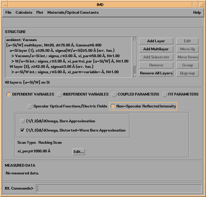
Figure 2.3.2 shows the main IMD widget as it appears when the DEPENDENT VARIABLES button is selected, and the Non-Specular Optical Functions button is selected.
Figure 2.3.2 The DEPENDENT VARIABLES / Non-Specular Optical Functions section of the main IMD widget.
For all computations, you must specify one or more incidence angles, and one or more photon wavelengths or energies. These two independent variables are always listed in the Independent Variables List, as shown in Figure 2.2.3
Figure 2.3.3 The main IMD widget as it appears when the INDEPENDENT VARIABLES button is selected.
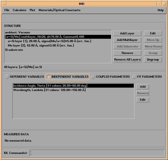
To specify angles and wavelengths (or energies), either double-click on the corresponding Independent Variables List element, or use the Edit button (to the right of the Independent Variables List) after selecting the variable you wish to edit.
The Incidence Angles and Wavelengths/Energies independent variables widgets are shown in the next two figures:
Figure 2.3.4 Angles widget
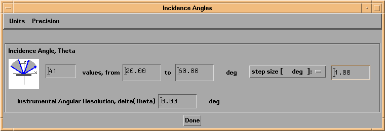
Figure 2.3.5 Wavelegths/Energies widget
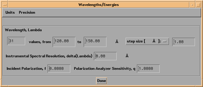
As can be seen from these figures, you can specify the desired number of values, the range of values, or the step size for angles and wavelengths (or energies.) (You can also select logarithmic steps, if desired, in which case the step size entry area disappears, as the step size is no longer constant.)
Additionally, if three or more angles (wavelengths/energies) are specified, you can specify the Instrumental Angular Resolution (Instrumental Spectral Resolution), in order to simulate finite instrumental resolution. For example, if you specify an Instrumental Angular Resolution of 0.5 degrees, then the optical functions you calculate will be convolved with a 0.5-degree-wide Gaussian function.
Note: Specifying instrumental resolution has no effect on the Electric Field Intensity calculations.
In the case of wavelengths/energies, you must also specify the Incident polarization factor, f, and the Polarization analyzer sensitivity, q. The quantity f is defined as the ratio (I(s)-I(p)) / (I(s)+I(p)), where I(s) and I(p) are the incident intensities of s and p polarizations. So for pure s-polarization, specify f=+1; for pure p-polarization specify f=-1, or for unpolarized incident radiation, specify f=0. The quantity q is defined as the sensitivity to s-polarization divided by the sensitivity to p-polarization. Specifying a value of q other than 1.0 could be used to simulate, for example, the reflectance you would measure using a detector that (for whatever reason) was more or less sensitive to s-polarization than to p-polarization.
Note: For specular optical functoins, the values of f and q that you specify only determine the values of the 'average' optical properties.
For example, the 'average' reflectance is given by:
R=(Rs*q*(1+f)+Rp*(1-f))/(f*(q-1)+(q+1)).
The average transmittance, absorptance, and electric field intensities are given by equivalent expressions. As mentioned above, the optical properties for the pure polarizations are always calculated.
Note: For non-specular reflected intensity calculations using the Born approximation, since there is coupling between s and p polarizations (in general), things are more complicated:
For an incident beam having a polarization factor f, the s-polarized and p-polarized components of the non-specular reflected intensity, (1/I0)dI/dOmega_s and (1/I0)dI/dOmega_p, respectively, are given by:
(1/I0)dI/dOmega_s=((1/I0)dI/dOmega_ss*(1+f) + (1/I0)dI/dOmega_ps*(1-f))/2
(1/I0)dI/dOmega_p=((1/I0)dI/dOmega_sp*(1+f) + (1/I0)dI/dOmega_pp*(1-f))/2
where
(1/I0)dI/dOmega_ss = reflected intensity component having s polarization, resulting from the fraction of the incident beam having s polarization
(1/I0)dI/dOmega_sp = reflected intensity component having s polarization, resulting from the fraction of the incident beam having p polarization
(1/I0)dI/dOmega_ps = reflected intensity component having p polarization, resulting from the fraction of the incident beam having s polarization
(1/I0)dI/dOmega_pp = reflected intensity component having p polarization, resulting from the fraction of the incident beam having p polarization
The 'average' reflected intensity, i.e., as measured with a detector having polarization sensitivity q (as defined above,) is then given by:
(1/I0)dI/dOmega_a=2*((1/I0)dI/dOmega_s*q + (1/I0)dI/dOmega_p)/(1+q)
Thus, the values of the s and p components of the scattered intensity depend on the specified value of f, while the 'average' scattered intensity depends on both f and q.
Use the Units and Precision menus to specify angle and photon units and precision, respectively. That is, you can choose to specify angles relative to normal incidence or relative to grazing incidence, and in degrees, arc-minutes, arc-seconds, or milliradians, and you can choose to specify photon wavelengths in angstroms, nanometers, microns, or cm-1, or photon energies in eV or keV.
In addition to angles and wavelengths (or energies), any of the (continuously variable) parameters that describe the structure can be designated as independent variables: optical constants, densities, compositions, layer thicknesses, interface widths, PSD parameters, graded interface parameters, etc. You can also specify the instrumental resolutions and polarization factors (f and q) as independent variables. Up to eight independent variables can be specified simultaneously.
To specify additional independent variables, press the Add button to the right of the Independent Variables List to bring up a menu of parameters available. Once you add a new independent variable to the Independent Variable List, you can edit the variable in the usual way: either by double-clicking or pressing the Edit button.
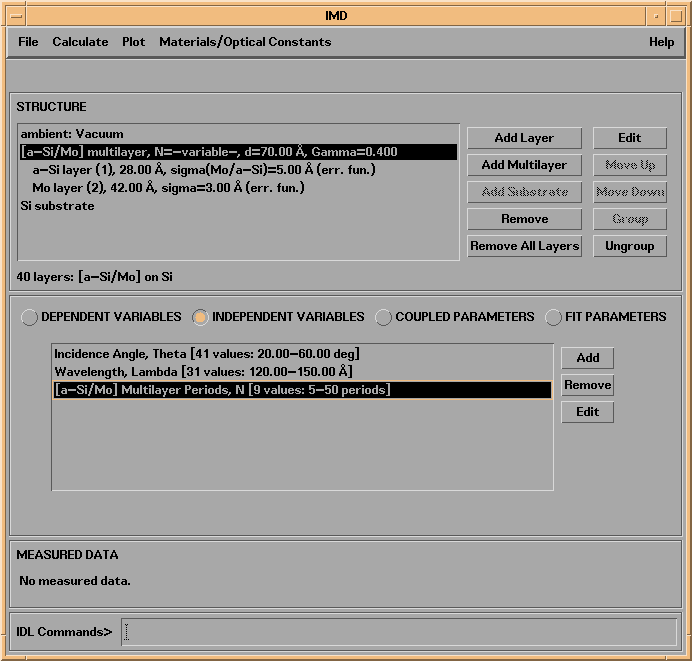
As an example, shown in Figure 2.3.6 is the independent variable widget that would result from specifying a multilayer period N to be an independent variable. In this case, I have selected 9 values of N, from 5 to 50. Note that in the Structure List, shown in Figure 2.3.7, the multilayer description line now reads N=-variable-, indicating that N is an independent variable. Other specific examples of specifying multiple independent variables will be presented in Section 2.5.
Figure 2.3.6 An independent variable widget corresponding to defining multilayer period N as an independent variable.

Figure 2.3.7 The main IMD widget showing the multilayer period N as an independent variable.
INDEPENDENT VARIABLES SPECIFIC TO ELECTRIC FIELD CALCULATIONS
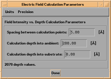
In the case of electric field intensity calculations, a third independent variable - depth, i.e., the position in the structure, measured from the top of the first layer - is always defined as well. This independent variable is not listed in the Independent Variables List. It is specified by pressing the button labelled Parameters... that appears when you select the Electric Fields dependent variable button. The depth variable is specified by three parameters, the spacing between calculation points, the calculation depth into the ambient, and the calculation depth into the substrate (if the substrate is present.) Note that the depth values are not equally spaced, as it is necessary to calculate the field intensities precisely at the interfaces between layers. So the specified spacing between calculation points represents an average value.
Figure 2.3.8 The Electric Field Calculation Parameters widget.
INDEPENDENT VARIABLES SPECIFIC TO NON-SPECULAR OPTICAL FUNCTIONS
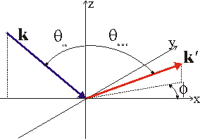
For non-specular computations, you must also specify the scattering angles and the type of `scan' you wish to model. Thus, when you select either the BA or DWBA functions as dependent variables, two additional independent variables will be defined: the first is related to the scattering angle, Thetaout, the second is the scattering plane azimuthal angle, phi. These angles are illustrated in Figure 2.3.9.
Figure 2.3.9 Scattering geometry associated with non-specular scattering.
Non-specular reflected intensity computations can be computed for any one of three different scattering geometries, or 'scans', as summarized in table 2.3.1 The three scan types - Rocking Scan, Detector Scan, and Offset Scan - are common to grazing incidence X-ray scattering measurements, but are equally valid for any wavelengths and over any range of incidence angles.
Table 2.3.1 Non-specular scattering scan types.
|
Scan Type |
Description |
| Rocking Scan | Detector fixed, sample rotated |
| Detector Scan | Sample fixed, detector rotated |
| Offset Scan | Sample and detector rotated simultaneously;
Detector offset from specular direction by a constant angle |
The way that you specify scattering angles in IMD depends on both the type of scan you have selected, and whether you choose to specify grazing incidence angles or normal incidence angles, as summarized in Table 2.3.2:
Table 2.3.2. Independent variable angle specification for non-specular scattering computations.
|
Scan Type |
Angle specified in IMD Incidence Angles independent variable widget |
Angle specified in IMD Scattering Angles independent variable widget |
| Rocking Scan, Normal Incidence | Theta =Thetain | Thetain+Thetaout |
| Rocking Scan, Grazing Incidence | Theta = 90 deg -Thetain | TwoTheta = 180 deg -Thetain-Thetaout |
| Detector Scan, Normal Incidence | Theta =Thetain | Thetain+Thetaout |
| Detector Scan, Grazing Incidence | Theta = 90 deg -Thetain | TwoTheta = 180 deg -Thetain-Thetaout |
| Offset Scan, Normal Incidence | Theta =Thetain | Delta(Thetaout) |
| Offset Scan, Grazing Incidence | Theta = 90 deg -Thetain | Delta(TwoTheta) |
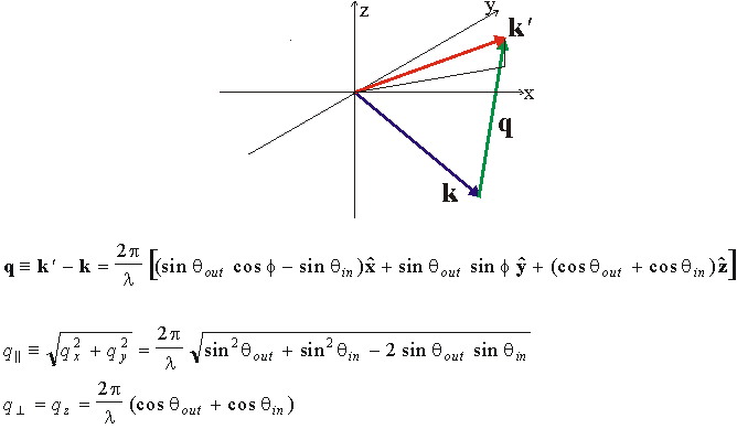
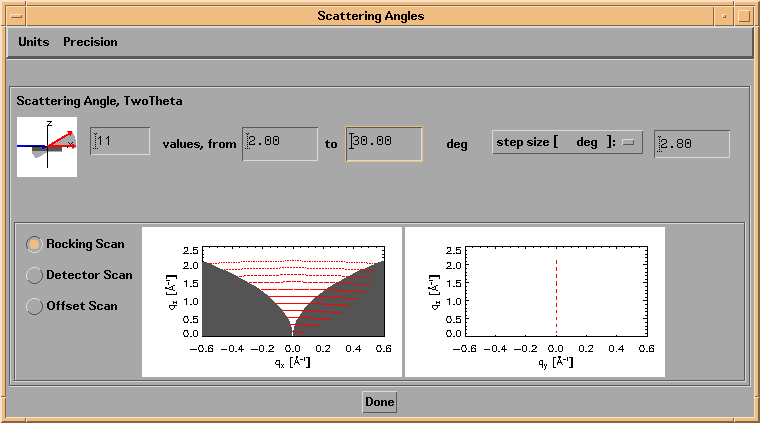
Shown in Figures 2.3.10 and 2.3.11 are the independent variable widgets associated with the scattering angle variable and the scattering plane azimuthal angle variable. Included on each widget is a schematic diagram illustrating the scattering geometry corresponding to the range of values you specify. In addition, the Scattering Angles widget includes plots of qx vs qz and qy vs qz, illustrating the corresponding scan trajectories in momentum space; the greyed regions on these plots indicate inaccessible regions of q-space, i.e., regions where either Thetain or Thetaout are greater than 90 degrees. The relationships between scattering angles and q-vectors are shown in Figure 2.3.12.
Figure 2.3.10. The Scattering Angles independent variable widget. In this case, a Rocking Scan has been selected for a single value of the scattering angle TwoTheta.
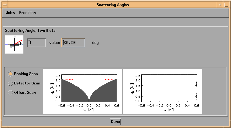
Figure 2.3.11. The Scattering Plane Azimuthal Angle independent variable widget.

Figure 2.3.12 Relationship between incidence and scattering angles and momentum vectors.
Although each of the three non-specular scan types refers to a one-dimensional scan, you are free to specify both multiple incidence angles and multiple scattering angles for any type of scan, in order to compute non-specular reflected intensity as a function of both angles. As a specific example, in the case of a Rocking Scan at grazing incidence, you can compute the non-specular reflected intensity for a range of incidence angles Theta, and for a single value of TwoTheta (as in Figure 2.3.10, for example,) or, you can compute the scattered intensity for both a range of Theta values and a range of TwoTheta values. In the latter case, the scattered intensity will be computed as a series of Rocking Scans, i.e., the scattered intensity will be computed as a function of Theta, for every value of TwoTheta you have specified. Figure 2.3.13 illustrates.
Note: The non-specular reflected intensity functions will be set to zero wherever either the incidence angle (Theta_in) or the scattering angle (Theta_out) exceeds 90 degrees.
Figure 2.3.13. The Scattering Angle independent variable widget for the case of a Rocking Scan when multiple values of the scattering angle TwoTheta have been specified.
Note: Because of the fact that the momentum transfer vector q depends on the wavelength, the incidence angle, and the two scattering angles, and because it is possible in IMD to vary any or all of these four parameters simultaneously, it is not possible to specify q-vectors directly. However, the results of your computations can be displayed as plots in momentum space, as will be described in Section 2.5.
It's possible in IMD to constrain individual layer or substrate parameters to be equal or proportional to other layer or substrate parameters, through the use of so-called 'Coupled Parameters'.
As an example, suppose you define a structure containing two layers, and you wish to set the interfacial width of layer A to be twice the interfacial width of layer B. As an alternative to entering directly the interface width values for each of the two layers, you can instead define a coupled parameter, such that the interface width of the A layer will always be equal to 2 times the value of the B layer interface width. The main advantage of using a coupled parameter in this case is that if you then define the 'source' of the coupled parameter - in this case the B layer interface width - to be an independent variable (or a fit parameter, as described in Section 3.2) , both parameter values can be varied simultaneously. In fact, multiple layer or structure parameters can all be coupled to the same 'source' parameter, allowing you to vary many parameters simultaneously, using only a single independent variable (or fit parameter.)
To define a coupled parameter, select the COUPLED PARAMETERS button on the main IMD widget, and then press the Add button in the Coupled Parameters region. (See Figure 2.3.14.) You will be presented with a list of available parameters that can be designated as coupled parameters. Choose one of these parameters. You will then be presented with a list of available 'source' parameters. Once you select the source parameter, a new Coupled Parameters widget will appear, as shown in Figure 2.3.15.
Figure 2.3.14. The main IMD widget as it appears when the COUPLED PARAMETERS button is selected.
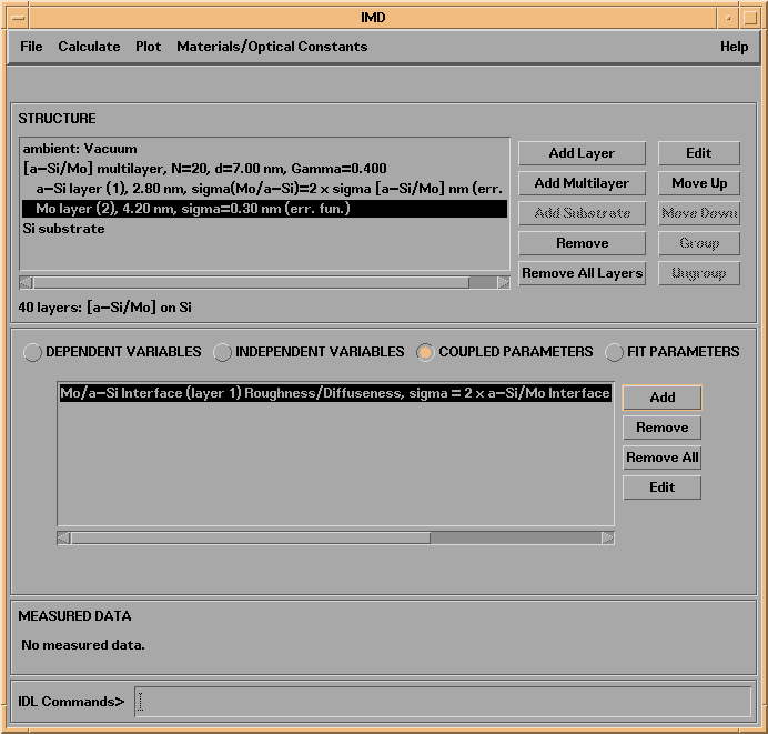
Figure 2.3.15. A Coupled Parameters widget.

On the Coupled Parameters widget you can enter the proportionality factor relating the source and destination parameters - a factor of 2 is shown in Figure 2.3.15 - and you can press the Change source parameter... button in order to (yes, you guessed it) change the source parameter.
The number of coupled parameters that can defined is limited only by the number of layers you define in the structure.
Note: Once a parameter is defined as (the destination parameter of) a coupled parameter, it's value can no longer be specified directly, nor can that parameter be defined as an independent variable or fit parameter.
See Section 2.5 for several examples illustrating the use of coupled parameters.