After the calculation is completed, the results will be saved to an IMD file automatically, unless you have disabled this feature in the File->Preferences->Auto-Save... menu option.
Note: Unless you disable auto-save, IMD will remember exactly how you left things the last time you ran IMD, so that you can continue right where you left off.
If you wish to save the results of different calculations in different IMD files for later use, use the File->Save as.. menu option. Saved IMD files can later be opened using the (you guessed it) File->Open... menu option.
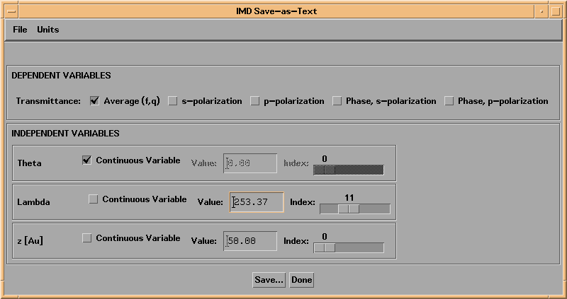
You can also save the results as plain text, if you wish, by selecting File->Save as Text... from the menu bar. You will be presented with a widget that allows you to specify which dependent variables you wish to save, and as a function of which independent variable, if there is more than one (multi-valued) independent variable available. For example, if you have calculated reflectance as a function of both incidence angle and wavelength, you must specify whether you wish to save reflectance vs. angle data at a specific wavelength, or reflectance vs. wavelength data at a specific angle. Figure 2.5.1 illustrates:
Figure 2.5.1 The IMD Save-as-Text widget associated with a transmittance calculation using three independent variables: angle, wavelength, and layer thickness.

After the calculation is completed, the results will be displayed graphically in an IMDXPLOT widget. The appearance of the IMDXPLOT widget depends on the dependent and independent variables you have specified, as will now be described.
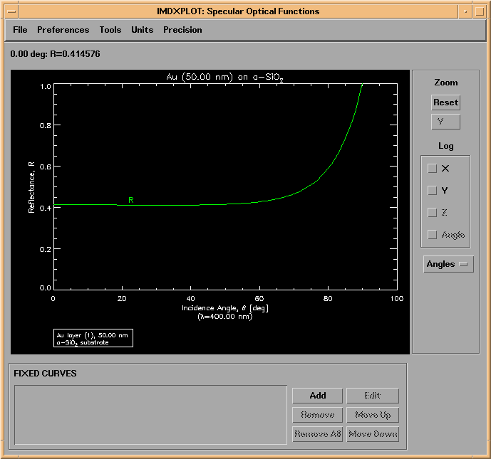
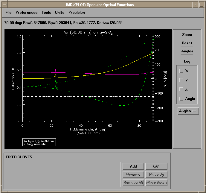
Shown in Fig. 2.5.2 is the IMDXPLOT widget that results from a calculation of reflectance vs incidence angle for a 50 nm gold film on an amorphous SiO2 substrate.
Figure 2.5.2 IMDXPLOT example showing the reflectance of a thin film on a substrate.
For each dependent variable selected in the DEPENDENT VARIABLES area of the main IMD widget, at least three quantities are actually calculated, as previously mentioned: the values of the property for pure s and pure p polarizations, as well as the 'average' value. In the case of reflectance and transmittance, the phases are calculated as well; in the case of reflectance, the ellipsometric psi and delta functions are also computed.
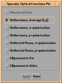
Shown in Figure 2.5.3 is the Plot Variables widget associated with the IMDXPLOT widget shown in Figure 2.5.2. This widget is accessible from the Preferences->Plot Variables... menu option on the IMDXPLOT widget. The default setting is to plot only the 'average' reflectance for the specified polarization parameters f and q, as shown:
Figure 2.5.3 IMDXPLOT Plot Variables widget
Shown in Figure 2.5.4 is the plot that results after selecting instead as plot variables R(s), R(p), and also the ellipsometric psi and delta functions. I have also changed the colors and linestyles of the different curves using the Preferences->Plot Variables Styles and Labels... option, and I have adjusted the axes using the Preferences->Axes Scaling... option. The cross-hairs at 79 degrees are due to the fact that I've also selected R(p) as the active 'cursor function'.
Figure 2.5.4 Plot after selecting several Plot Variables.
You can use your mouse to zoom in on a particular region of the plot. Alternatively, more precise axis scaling can be adjusted from the menu items on the IMDXPLOT widget; many other aspects of the plot can be adjusted as well: colors, linestyles, thicknesses, plotting symbols, labels and label placement, character size, etc. Once you have adjusted the plot to your liking, you can print it using the File->Print menu option.
Note: You can change the default background and plot color, by setting the values of the IDL graphics system variables !p.background and !p.color. For example, to produce a plot with black lines on a white background (instead of the default white plot on a black background), set !p.background=255 and !p.color=0, prior to plotting your results with IMDXPLOT. You can enter these commands either at the IDL prompt, or from within the IDL Commands area of the main IMD widget.
Note: Use the droplist widget (labeled Angles in Figure 2.5.4, for example) to the right of the plot area on an IMDXPLOT widget to display an optical function vs. q (momentum) rather than incidence or scattering angle.
As a second, and somewhat more complicated example, shown in Figures 2.5.5 and 2.5.6 are IMDXPLOT widgets corresponding to the results of a calculation of the reflectance of a carbon film vs. angle of incidence, wavelength, and film thickness. There are many different ways to display the results of such a multi-variable calculation. In Figure 2.5.5, I have chosen to display a 1D plot showing Reflectance vs. Incidence Angle. Thus, the Continuous Variable box next to the word Theta is checked, signifying that Theta (incidence angle) is a continuous plot variable, whereas the boxes next to Lambda and z[a-C] are unchecked, indicating that these parameters are discrete variables. That is, the plot shows the reflectance-vs-angle curves for whichever value of Lambda is entered in the box labeled 'Value' to the right of the word Lambda. Alternatively, you can position the slider labelled Index to view R-vs-Theta curves for different wavelength array indices. On the other hand, in Figure 2.5.6, I've designated both angle and wavelength as continuous variables, and have displayed the results as a 2D surface plot.
Figure 2.5.5 A 1D plot showing the reflectance of a carbon film as a function of incidence angle.
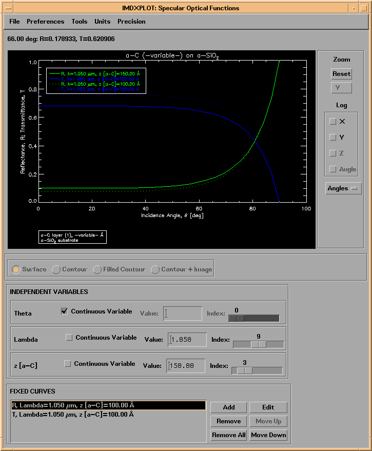
Figure 2.5.6 A 2D surface plot, showing the reflectance of the same carbon film, as a function of both angle and wavelength, and for two different film thicknesses.
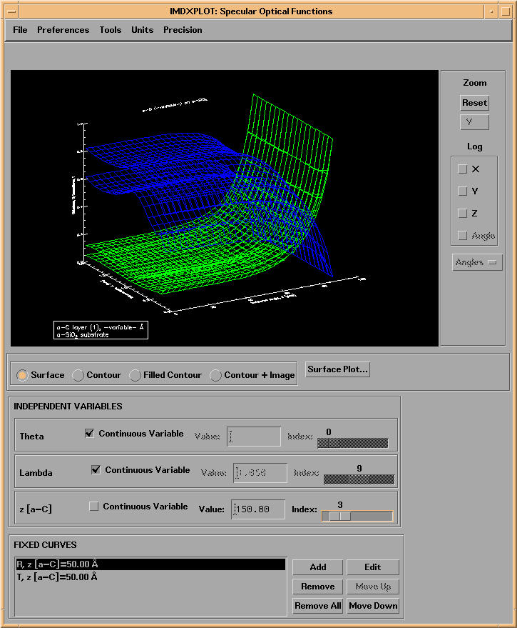
The way to display more than one curve at a time, as in Figures 2.5.5 and 2.5.6, is to add "Fixed Curves" to the plot. By pressing the Add button in the FIXED CURVES area of the IMDXPLOT widget, the currently displayed curves will be added to the list of "Fixed" curves. The appearance (i.e., color, linestyle, etc.) of each fixed curve can be edited by selecting the fixed curve in the usual way: either double-clicking on the line in the Fixed Curve List area, or by selecting the curve you wish to edit and pressing the Edit button. You can also change the label for the curve, and you can choose to use 'curve labels' (as in Figure 2.5.4, for example), or use a legend (as in Figure 2.5.5.) If you choose to use a legend, you can adjust the order in which the curves are listed in the legend by using the Move Up and Move Down buttons in the FIXED CURVES area. You can add as many as 30 Fixed Curves to the plot.
Note: You can have more than one IMDXPLOT widget open at a time. This makes it easier to compare the results from different types of calculations. But, this also means that any changes you make in the main IMD widget (i.e., changes to the structure or to the dependent or independent variables) will only affect future instances of IMDXPLOT. So once a calculation is completed and the IMDXPLOT widget is created, you cannot change the data associated with that instance of IMDXPLOT (although you can always change the plot appearance, using the IMDXPLOT Preferences options.) This also means that any changes you make to the plot using the IMDXPLOT Preferences options will only affect that instance if IMDXPLOT.
To specify preferences that you want to apply to all future instances of IMDXPLOT, use the Plot->Global Plot Preferences... option from the main IMD widget menu bar.
Also, you can save the plot appearance changes (and fixed curves) you might have made in IMDXPLOT along with the data by using the File->Save... option from the IMDXPLOT menu bar.
You can use the Tools->Statistics/Region-of-Interest IMDXPLOT menu option to define a region-of-interest, and compute a variety of statistics for whatever optical functions are currently displayed, including measured data. (Loading your measured data into IMD will be discussed in Chapter 3.)
For example, shown in Figure 2.5.7 is the calculated X-ray reflectance of a W/Cr bilayer film, plotted as a function of q_z; the two dashed vertical lines on this plot refer to the region-of-interest that was defined on the Statistics widget shown in Figure 2.5.8. Note that this region-of-interest was digitized to encompass one period of the high-frequency modulation visible in the reflectance curve. In this example, this modulation is due to the total film thickness; thus, the Corresponding layer thickness indicated in the Statistics widget of Figure 2.5.8 is an estimate of the total film thickness. This technique is especially useful with measured data when trying to fit X-ray reflectance data in order to determine film thicknesses. (The data used to produce Figure 2.5.7 is contained in the file examples.dir/WCr_bilayer.dat.)
Figure 2.5.7. The calculated X-ray reflectance of a W/Cr bilayer film. The dashed vertical lines refer to the region-of-interest indicated in Figure 2.5.8.
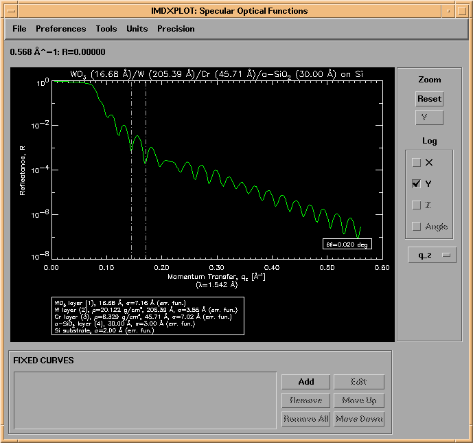
Figure 2.5.8. The Statistics widget associated with the IMDXPLOT widget shown in Figure 2.5.7
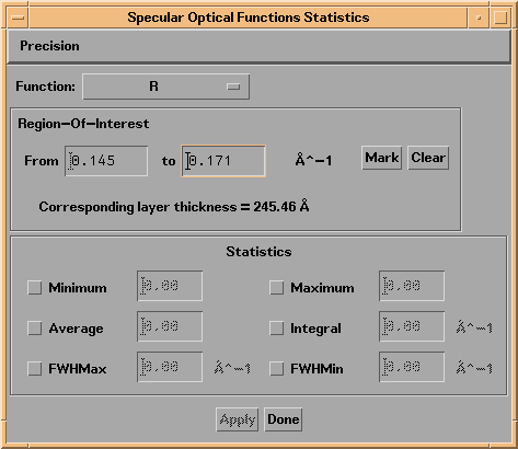
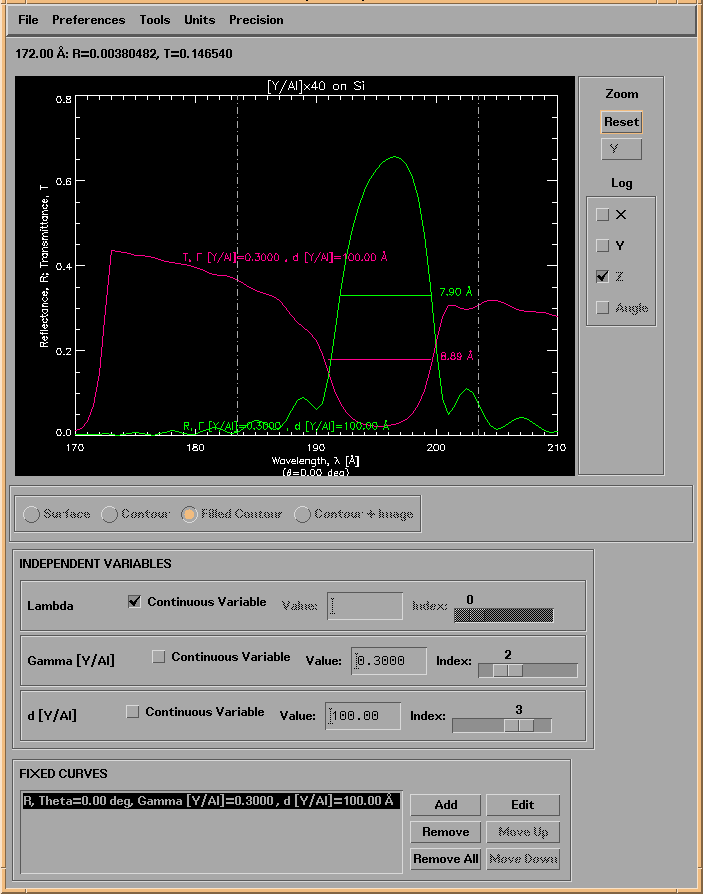
As can be seen in the Statistics widget of Figure 2.5.8, six different statistics can be determined: Minimum, Maximum, Average, Integral, Full-Width-Half-Max, and Full-Width-Half-Min (which refers to the width of an 'absorption' feature.) To illustrate, shown in Figure 2.5.9 is the reflectance and transmittance of a Y/Al multilayer film, with the width of the Bragg peak in both functions indicated.
FIgure 2.5.9. The reflectance and transmittance of a Y/Al multilayer. The FWHMax of the reflectance, and the FWHMin of the transmittance curves are indicated.
Note: the statistics you select are computed only over the region-of-interest you define.
Note: to display statistics for more than one function simultaneously, as in Figure 2.5.9, you will need to compute the statistics for one function at a time, and then display each function as a Fixed Curve, as described above.
Included here are a few more examples illustrating some of the types of computations and visualizations that are possible in IMD.
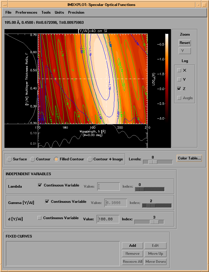
Shown in Figure 2.5.10 is the reflectance and transmittance of the same Y/Al multilayer used in Figure 2.5.9. In this case, however, these specular optical functions are displayed as a function of both wavelength and multilayer thickness ratio (Gamma) as color contour plots: contours of constant reflectance are shown in green, contours of constant transmittance are shown in blue, and both sets of contours are overlayed on the a filled contour plot of the reflectance The grey 1D plots below and to the left of the contour plot are 'live' plots that vary as you move the cursor over the contour plot. (The data used to create this plot is in the file called examples.dir/YAl.rt.dat.)
Figure 2.5.10. Reflectance and transmittance contours for a Y/Al multilayer film, as a function of wavelength and layer thickness ratio.
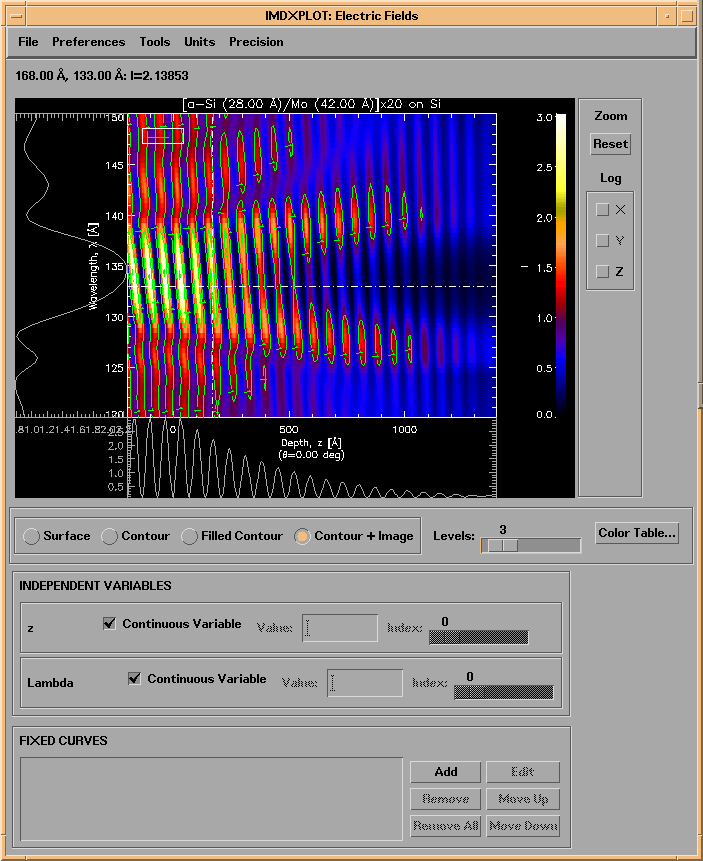
Similarly, shown in Figure 2.5.11 are the electric field contours for a Mo/Si multilayer film, as a function of wavelength and depth into the film (see the file examples.dir/SiMo.fields.dat):
Figure 2.5.11. Electric field intensity contours for a Mo/Si multilayer film.
The next example, shown in Figure 2.5.12 (and contained in the file examples.dir/CNi.graded.dat,) is the grazing incidence X-ray reflectance vs. energy of a graded C/Ni multilayer film, showing the effect of interface roughness/diffuseness on the specular reflectance. This calculation was made by defining two coupled parameters (see Section 2.3): the Ni layer thickness was set to be 0.8 times the C layer thickness (which was graded), and the Ni layer interface width was set equal to the C layer interface width, which itself was defined as an independent variable.
Figure 2.5.12. The grazing incidence X-ray reflectance of a graded C/Ni multilayer, as a function of interface width.
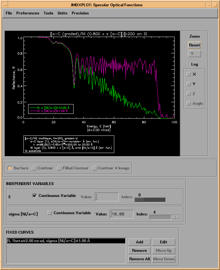
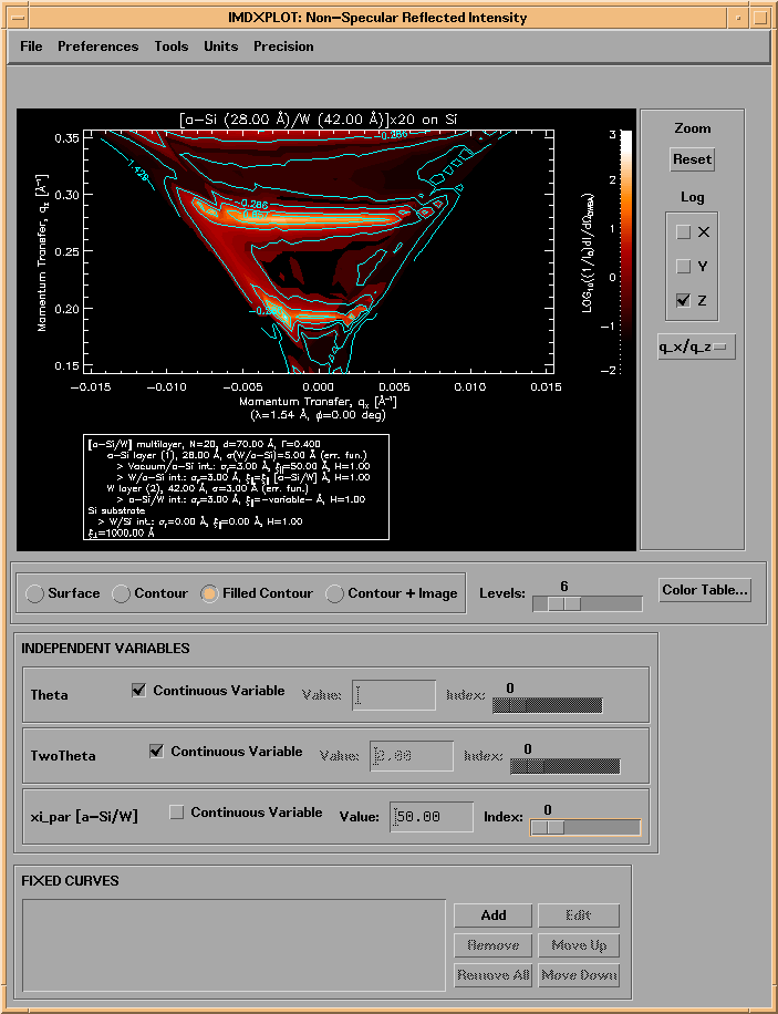
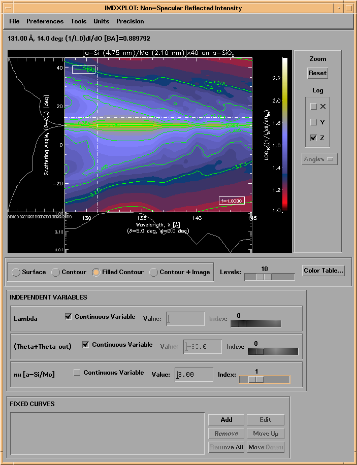
Figure 2.5.13 shows the result of a calculation of the non-specular reflected intensity for a Mo/Si multilayer film, near normal incidence in the soft X-ray region, computed using the Born approximation vector theory. The Omega/nu/n PSD model was used, and the PSD parameters of the Mo-on-Si interface were coupled to those of the Si-on-Mo interface; the Si-on-Mo relaxation coefficient, nu, was defined as an independent variable. Contours of constant intensity as a function of wavelength and scattering angle are superimposed on a filled color contour plot, and 1D slices are shown below and to the left of the contour plot. (See the file examples.dir/SiMo.ns_ba.dat.)
Figure 2.5.13. The non-specular reflected intensity for a Mo/Si multilayer film near normal incidence, computed using the BA theory (see Section 2.3.)
The last example, shown in Figure 2.5.14, is a plot in q-space of the grazing incidence, non-specular reflected X-ray intensity for a W/Si multilayer calculated with the DWBA theory, as a function of the lateral correlation length. The correlation length of the Si-on-W interface was coupled to that of the W-on-Si interface for this calculation. (See the file examples.dir/SWi.ns_dwba.dat.)
Figure 2.5.14. The non-specular reflected intensity for a W/Si multilayer film near grazing incidence, computed using the DWBA theory (see Section 2.3.)
