The abbreviated discussion of confidence intervals presented in this section is based largely on the methods described in references [16] and [17]. Please consult those papers for a full discussion.
To quote Lampton, et al., "In parameter estimation, it is the range of parameter values to which a theory is restricted that is the useful result of an experiment. The discrete best-fitting values of the parameters are essentially statistical artifacts subject to a variety of correlated random errors originating in the counting statistics of the original data. If an experiment could be repeated without systematic changes, best-fitting parameter values would differ, while their properly derived allowed ranges will overlap."
Once you have performed a fit, IMD can compute independent and joint confidence interval estimates on the fit parameters. The confidence intervals are estimated by computing the value of the Chi^2 statistic on a grid of points in parameter-space. Although there is no limit on the number of fit-parameters you can select when performing curve-fitting in IMD, due to the limit of 8-dimensional arrays imposed by IDL, you can only compute 8-dimensional confidence intervals. (If this is a problem for you, then you're probably doing something you shouldn't be doing anyway.)
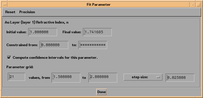
To compute confidence intervals, you must first designate which fit parameters are to be included in the parameter space to be examined. So, for each parameter of interest, you must check the box labelled Compute confidence intervals for this parameter, in the associated Fit Parameter widget. Shown in Figure 3.4.1 is the Fit Parameter widget for the refractive index, n of the Au film in the example of the previous section.
Figure 3.4.1 Fit Parameter widget for refractive index, n

For each fit parameter you select, you must specify the parameter grid over which the Chi^2 statistic is to be computed. To illustrate, in figure 3.4.1, because the best fit value for n is approximately 1.66, I have selected 21 parameter values, ranging from n=1.5 to 2.0. Similarly, I have selected 21 values for k, ranging from 1.9 to 2.1 (not shown.)
Once you have completed the parameter grid specifications for all fit parameters of interest, select the Calculate->Compute Confidence Intervals option from the main IMD widget. IMD will then iterate through each of the parameter values throughout the parameter-space grid you have defined, and compute the value of Chi^2.
The actual method used to compute Chi^2 at each point in the parameter space you have defined depends on what fraction of the fit parameters you have specified for confidence interval generation. That is, if you have elected to compute confidence intervals for all of the fit parameters used to perform the fit, then IMD will simply compute the value of the optical function for each of the parameter values, and compare it with the measured data in order to compute the value of Chi^2 at that point in parameter space. On the other hand, if you have selected only some of the parameters for confidence interval generation, then IMD will perform a non-linear, least-squares fit to the data at each of the points in the parameter-space grid you have defined, with the remaining fit parameters used as adjustable parameters to minimize Chi^2 at that point in parameter space. This latter option is useful if, for example, your fit parameters consist of a mix of 'interesting' and 'uninteresting' parameters. As an example, if you have derived optical constants, n and k, from reflectance vs. incidence angle data, and have also used a Reflectance Offset as a fit parameter to account for some offset in your data, then you might wish to compute confidence intervals for n and k, but not for the Reflectance Offset.
After the calculation is completed, the results will be saved to an IMD file automatically, unless you have disabled this feature in the File->Auto-Save Preferences menu.
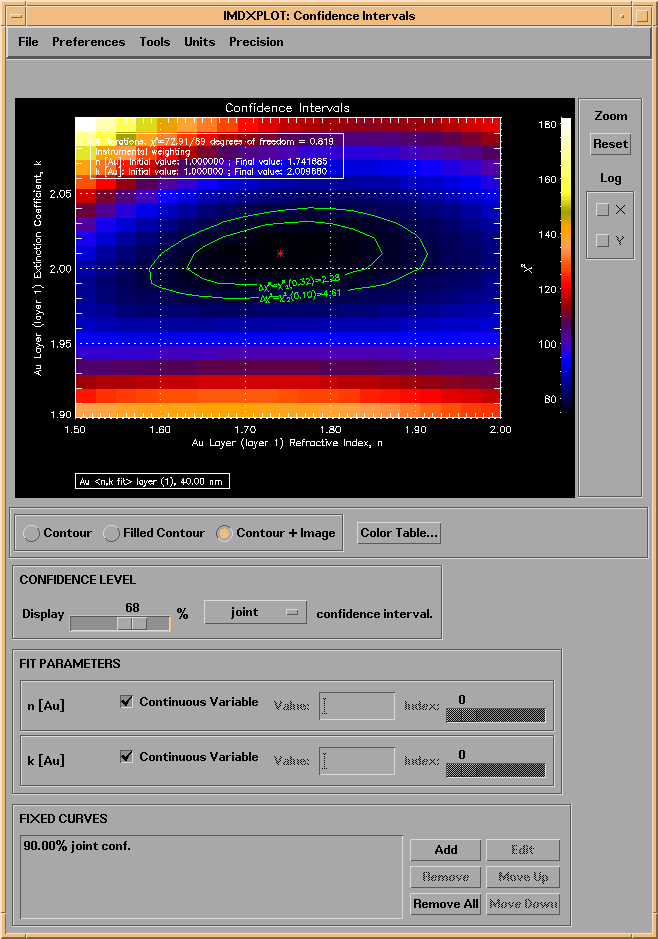
The confidence intervals will be displayed in another IMDXPLOT widget, as shown, for example in Figure 3.4.2:
Figure 3.4.2 Confidence Intervals plot.

By checking the Continuous Variable boxes next to each of the fit parameters (in the FIT PARAMETERS area of the IMDXPLOT widget,) you can display either 1D plots of Chi^2 versus the parameter value, or 2D contour plots showing contours of constant Chi^2. You can use the Value and Index widgets for non-continuous fit parameters to display Chi^2 plots for discrete parameter values, and you can used the FIXED CURVES buttons to overlay multiple confidence intervals on the same plot.
The area of the IMDXPLOT widget labelled CONFIDENCE LEVEL allows you to adjust which confidence level is displayed, and, if you have computed confidence intervals for more than one parameter, whether independent or joint confidence intervals are shown. These adjustments determine the value of Delta(Chi^2) that is displayed on the plots. That is, the confidence interval corresponds to the region in parameter space for which the value of the Chi^2 statistic is less than the minimum value (i.e., the value at the best-fit point) plus an amount Delta(Chi^2). For example, if you have computed confidence intervals for 2 fit parameters, then the 68% joint confidence interval corresponds to Delta(Chi^2) = 3.5, which is the value of the Chi^2 function for 2 parameters with significance 1-.68=.32. (Please refer to Lampton et al. for further details.)
Shown in Figure 3.4.2 are 68% and 90% joint confidence intervals for n and k, for the example we have been discussing. The meaning of these contours is the following: there is a 68% (90%) probability that the true values of n and k both lie within the green (red) region displayed in the figure.